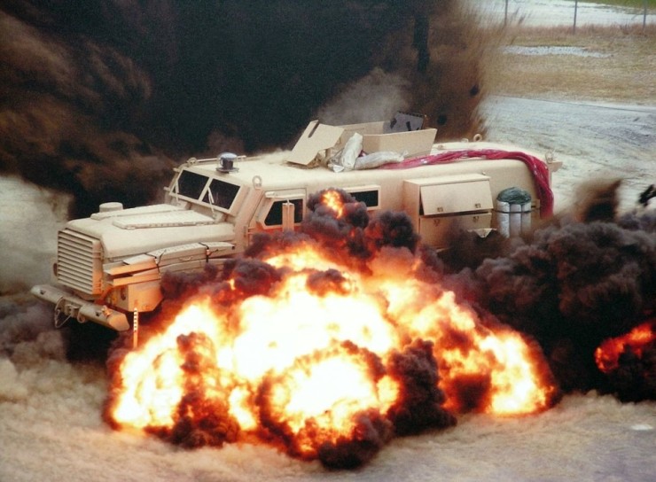
프로젝트에서 폭발에 대해서 탐지기능을 갖추어야 한다.
이것을 진행하기위해서,
먼저, 폭발에 대한 이미지를 먼지/화염으로 각각 100장 수집하고 레이블링을 해보자
1. 이미지 수집
구글에서 이미지를 쉽게 긁어올 수 있는 도구가 없을까를 생각했다. 여기서 쉽게라는 것은 내가 화재라는 키워드를 주면 화재로 검색되어져 나오는 이미지를 다운로드 해주는 도구를 생각 했었다. 하지만, 키워드에 대한 이미지가 적절한 것인지에 정확성이 부족할 것 같다는 생각이 문득 들었다. 결국에는 사람이 이미지를 보고 원하는 이미지라는 것을 판단해야 하는 과정이 필요할 수 밖에 없는 것일까? 여기에는 많은 궁금점이 생긴다. (※ TODO 나보다 뛰어난 사람들이 저문제를 어떻게 해결 했는지 또는 해결해 나가는지 주기적으로 모니터링 할 필요가 있다는 생각이든다.)
여하튼, 현재의 나의 정보로는 적당한 생각이 들지 않아서 필요한 이미지에 대한 URL을 수집하여 URL을 통해 이미지를 다운로드하는 유틸리티(TODO) 정도를 만들어보려고 한다.
※정정 필요한 도구를 만들기전에 잘만들어져 있는 도구를 찾는 것을 먼저 해보자. 있다면 그 도구를 잘 사용해보고 불편하거나 버그가 있으면 PR 해보기
1.1 이미지 수집 도구
가. google-image-crawler
github: https://github.com/walkoncross/google-image-crawler-zyf
나. google-images-download
github: https://github.com/hardikvasa/google-images-download
다. icrawler
github: https://github.com/hellock/icrawler
docu: http://icrawler.readthedocs.io/en/latest/index.html
라. image donwloader in chrome plug-in
url: https://chrome.google.com/webstore/search/image%20downloader
위의 도구들을 이용하면 원하는 키워드에 다양한 옵션들을 설정하여 구글이미지를 다운로드 받을 수 있다. 하지만 여기서 또 여전히 의문점이 있다. 특정 키워드로 다운 받은 이미지가 내가 원하는 이미지가 맞는지 확인이 필요하다는 것이다.
실제로 저러한 도구를 이용하여 다운로드 받아보니, 어떤 이미지는 "워터망킹 되어서 삭제", "키워드랑 전혀 연관이 없어서 삭제", "이미지가 너무 흐릿해서 삭제", "실물 사진이 필요한데 사람이 만들어낸 그림(?) 이라서 삭제" 등등 이슈가 있었다.
여기서 다음 스텝으로 어떻게 해야할지 결정해야 겠다.
a. 현재 상태에서 내가 직접눈으로 불필요한 것들을 지운다.
- 이렇게 하면 지금 당장은 빠르지만 앞으로 같은일이 반복되었을때 같은 현상을 겪게 된다.
b. 구글 서칭 기법중 또는 옵션중에서 정확도를 높일수 있는 방법이 있는지 찾아본다.
- 이거는 조금 검색해보면 검색 방법들이 나올 수 있을것 같다. 하지만 검색 방법을 찾는다면, 내가 다운로드 받은 도구중에 하나를 선택해서 저 검색 기법들을 적용할 수 있는지 확인하고 개발해야 한다.
c. 나보다 경험을 더 많이 갖고 있는 AI를 하고 있는 사람들이 이미지 수집을 어떻게 하고 있는지 알아보고 그러한 조사중에 위의 문제를 해결할 수 있는 스마트한 방법 및 도구가 있는지 찾아본다.
- 이렇게 하면 "시간이 얼마나 걸릴지", "정말로 존재하는 것인지" 등의 의문을 갖으며 진행하게 될것 같다. 지인찬스를 한번 쓰는게 나을지도 모르겠다. 혹여나 찾으면 있다면 앞으로의 진행이 몇배는 빨라질거 같다.
d. 아! 갑자기 google vision api가 생각 났다. 내가 원하는 explosion이 라벨링이 되어 있다. 그렇다는 것은 어딘가에 이미지셋으로 존재 한다는 말이다. imagenet, coco 등등의 이미지를 갖고있는 진영에 대한 조사를 해보는게 좋을것 같다.
- 앞으로도 특정 오브젝트에 대한 이미지셋이(특이하지 않은) 필요할 예정이기 때문에 이방법을 선행하는게 좋겠다.
가. google-image-crawler
Image Donw load config.json 설정
|
|
{
"save_dir": "./downloads/",
"num_downloads_for_each_class": 200,
"search_file_type": "jpg",
"search_keywords_dict": {
"millitary": [
"millitary explosion"
]
},
"search_cdr_days": 60,
"output_prefix": "download_urls",
"output_suffix": "google"
}
|
cs |
Download Image
현재 디렉토리 구조
|
|
Object-Detection
-images/
--test/
--train/
--...yourimages.jpg
|
cs |
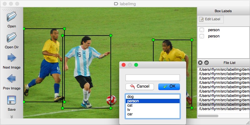
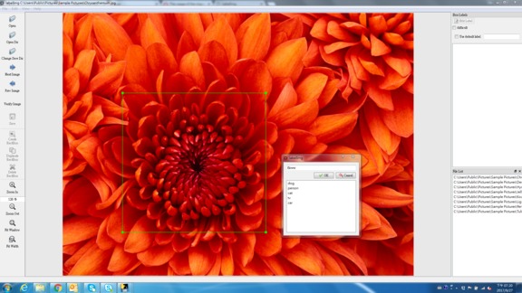
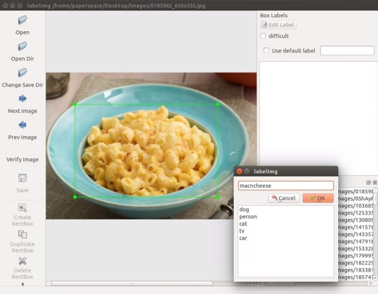
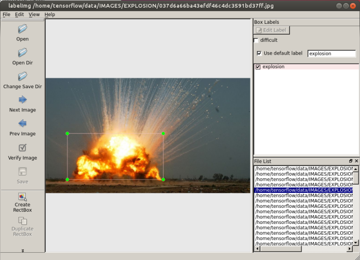
2. 이미지 라벨링
2.1 라벨링 도구
a. labelImg
github: https://github.com/tzutalin/labelImg
b. FastAnnotationTool
github: https://github.com/christopher5106/FastAnnotationTool
c. ImageMagick
url: http://imagemagick.org/script/download.php
a. 사용
Annotation.xml
|
|
<annotation>
<folder>EXPLOSION</folder>
<filename>f619a2dd1405af1e0118bd7700f84af4.jpg</filename>
<path>/home/tensorflow/data/IMAGES/EXPLOSION/f619a2dd1405af1e0118bd7700f84af4.jpg</path>
<source>
<database>Unknown</database>
</source>
<size>
<width>1920</width>
<height>1200</height>
<depth>3</depth>
</size>
<segmented>0</segmented>
<object>
<name>explosion</name>
<pose>Unspecified</pose>
<truncated>0</truncated>
<difficult>0</difficult>
<bndbox>
<xmin>149</xmin>
<ymin>112</ymin>
<xmax>1286</xmax>
<ymax>1031</ymax>
</bndbox>
</object>
</annotation>
|
cs |
현재 디렉토리 구조
|
|
Object-Detection
-images/
--test/
--train/
--...yourimages.jpg
--...yourimages.xml
|
cs |
3. 보유하고 있는 데이터를 train/test sample로 나누기
아래의 디렉토리 구조를 생성하고, 보유하고 있는 데이터를 train/test를 나눈다.
|
|
Object-Detection
-images/
--test/
---testingimages.jpg
---testingimages.xml
--train/
---trainingimages.jpg
---trainingimages.xml
--...yourimages.jpg
--...yourimages.xml
|
4. 학습을 위한 TF Records 변환
① xml 파일을 csv 파일로 변환
|
|
def main():
for directory in ['train','test']:
image_path = os.path.join(os.getcwd(), 'images/{}'.format(directory))
xml_df = xml_to_csv(image_path)
xml_df.to_csv('data/{}_labels.csv'.format(directory), index=None)
print('Successfully converted xml to csv.') |
cs |
생성된 CSV 파일을 Object-Detection 디렉토리에 data 디렉토리를 생성하고, data 디렉토리로 csv 파일을 옮긴다. 그리고 Object-Detection 디렉토리에 training 디렉토리를 생성한다. 지금까지의 디렉토리 구조는 아래와 같다.
Object-Detection
-data/
--test_labels.csv
--train_labels.csv
-images/
--test/
---testingimages.jpg
---testingimages.xml
--train/
---trainingimages.jpg
---trainingimages.xml
--...yourimages.jpg
--...yourimages.xml
-training
-xml_to_csv.py |
cs |
② 이제 CSV 파일을 TFRecord파일로 변환
generate_tfrecord.py
|
|
# TO-DO replace this with label map
def class_text_to_int(row_label):
if row_label == 'explosion':
return 1
else:
None |
cs |
이제 generate_tfrecord.py 스크립트를 수행한다. train TFRecord와 test TFRecord를 위해 두번 수행하게 된다.
train TFRecord:
|
|
python generate_tfrecord.py --csv_input=data/train_labels.csv --output_path=data/train.record
|
cs |
test TFRecord:
|
|
python generate_tfrecord.py --csv_input=data/test_labels.csv --output_path=data/test.record |
현재 디렉토리:
Object-Detection
-data/
--test.record
--test_labels.csv
--train.record
--train_labels.csv
-images/
--test/
---testingimages.jpg
---testingimages.xml
--train/
---trainingimages.jpg
---trainingimages.xml
--...yourimages.jpg
--...yourimages.xml
-training
-xml_to_csv.py |
5. 학습에 사용할 모델 고르기
먼저 checkpoint 와 configuration 파일을 다운 받는다.
I am going to go with mobilenet, using the following checkpoint and configuration file
wget https://raw.githubusercontent.com/tensorflow/models/master/object_detection/samples/configs/ssd_mobilenet_v1_pets.config
wget http://download.tensorflow.org/models/object_detection/ssd_mobilenet_v1_coco_11_06_2017.tar.gz
You can check out some of the other checkpoint options to start with here.
models/object_detection 디렉토리에서 ssd_mobilenet_v1을 가져와서 training 디렉토리에 놓는다.
ssd_mobilenet_v1_pets.config을 우리 환경에 맞게 그리고 여러 하이퍼 파라미터들을 조정 할 수 있다.
여기에서는 우리 환경에 맞게 설정해야할 몇몇 값들을 수정한다.
Put the config in the training directory, and extract the ssd_mobilenet_v1 in the models/object_detection directory
In the configuration file, you need to search for all of the PATH_TO_BE_CONFIGURED points and change them. You may also want to modify batch size.
Currently, it is set to 24 in my configuration file. Other models may have different batch sizes.
If you get a memory error, you can try to decrease the batch size to get the model to fit in your VRAM.
Finally, you also need to change the checkpoint name/path, num_classes to 1, num_examples to 12,
and label_map_path: "training/object-detect.pbtxt"
- 클래스가1개 이기때문에 num_classes를 1로 설정
- batch size는 메모리 여건에 따라서 조정
- fine_tune_checkpoint 경로 변경
- 학습 횟수가 디폴트로 20만번으로 되어있다. 상황에 따라서 num_steps을 조정
- train_input_reader의 input_path, label_map_path 경로 변경
- eval_input_readerinput_path, label_map_path 경로 변경
- TODO 기타 설정 값들에 대한 정리 자료 작성 필요
It's a few edits, so here is my full configuration file:
# Users should configure the fine_tune_checkpoint field in the train config as
# well as the label_map_path and input_path fields in the train_input_reader and
# eval_input_reader. Search for "${YOUR_GCS_BUCKET}" to find the fields that
# should be configured. model {
  ssd {
    num_classes: 1
    box_coder {
      faster_rcnn_box_coder {
        y_scale: 10.0
        x_scale: 10.0
        height_scale: 5.0
        width_scale: 5.0
      }
    }
    matcher {
      argmax_matcher {
        matched_threshold: 0.5
        unmatched_threshold: 0.5
        ignore_thresholds: false
        negatives_lower_than_unmatched: true
        force_match_for_each_row: true
      }
    }
    similarity_calculator {
      iou_similarity {
      }
    }
    anchor_generator {
      ssd_anchor_generator {
        num_layers: 6
        min_scale: 0.2
        max_scale: 0.95
        aspect_ratios: 1.0
        aspect_ratios: 2.0
        aspect_ratios: 0.5
        aspect_ratios: 3.0
        aspect_ratios: 0.3333
      }
    }
    image_resizer {
      fixed_shape_resizer {
        height: 300
        width: 300
      }
    }
    box_predictor {
      convolutional_box_predictor {
        min_depth: 0
        max_depth: 0
        num_layers_before_predictor: 0
        use_dropout: false
        dropout_keep_probability: 0.8
        kernel_size: 1
        box_code_size: 4
        apply_sigmoid_to_scores: false
        conv_hyperparams {
          activation: RELU_6,
          regularizer {
            l2_regularizer {
              weight: 0.00004
            }
          }
          initializer {
            truncated_normal_initializer {
              stddev: 0.03
              mean: 0.0
            }
          }
          batch_norm {
            train: true,
            scale: true,
            center: true,
            decay: 0.9997,
            epsilon: 0.001,
          }
        }
      }
    }
    feature_extractor {
      type: 'ssd_mobilenet_v1'
      min_depth: 16
      depth_multiplier: 1.0
      conv_hyperparams {
        activation: RELU_6,
        regularizer {
          l2_regularizer {
            weight: 0.00004
          }
        }
        initializer {
          truncated_normal_initializer {
            stddev: 0.03
            mean: 0.0
          }
        }
        batch_norm {
          train: true,
          scale: true,
          center: true,
          decay: 0.9997,
          epsilon: 0.001,
        }
      }
    }
    loss {
      classification_loss {
        weighted_sigmoid {
          anchorwise_output: true
        }
      }
      localization_loss {
        weighted_smooth_l1 {
          anchorwise_output: true
        }
      }
      hard_example_miner {
        num_hard_examples: 3000
        iou_threshold: 0.99
        loss_type: CLASSIFICATION
        max_negatives_per_positive: 3
        min_negatives_per_image: 0
      }
      classification_weight: 1.0
      localization_weight: 1.0
    }
    normalize_loss_by_num_matches: true
    post_processing {
      batch_non_max_suppression {
        score_threshold: 1e-8
        iou_threshold: 0.6
        max_detections_per_class: 100
        max_total_detections: 100
      }
      score_converter: SIGMOID
    }
  }
} train_config: {
  batch_size: 10
  optimizer {
    rms_prop_optimizer: {
      learning_rate: {
        exponential_decay_learning_rate {
          initial_learning_rate: 0.004
          decay_steps: 800720
          decay_factor: 0.95
        }
      }
      momentum_optimizer_value: 0.9
      decay: 0.9
      epsilon: 1.0
    }
  }
  fine_tune_checkpoint: "ssd_mobilenet_v1_coco_11_06_2017/model.ckpt"
  from_detection_checkpoint: true
  data_augmentation_options {
    random_horizontal_flip {
    }
  }
  data_augmentation_options {
    ssd_random_crop {
    }
  }
} train_input_reader: {
  tf_record_input_reader {
    input_path: "data/train.record"
  }
  label_map_path: "data/object-detection.pbtxt"
} eval_config: {
  num_examples: 40
} eval_input_reader: {
  tf_record_input_reader {
    input_path: "data/test.record"
  }
  label_map_path: "training/object-detection.pbtxt"
  shuffle: false
  num_readers: 1
}
TODO pbtxt 역할에 대해서 정리하기.
vi object-detection.pbtxt
Inside training dir, add object-detection.pbtxt:
item { id: 1
name: 'macncheese'
}
현재 디렉토리:
Object-Detection -data/ --test.record
--test_labels.csv --train.record
--train_labels.csv -images/
--test/
---testingimages.jpg
---testingimages.xml
--train/
---trainingimages.jpg
---trainingimages.xml
--...yourimages.jpg
--...yourimages.xml -ssd_mobilenet_v1_coco_11_06_2017 -training
-xml_to_csv.py |
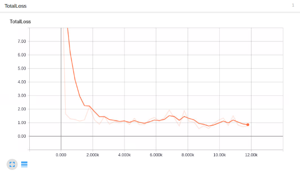
6. 학습 시키기(Train)
학습이 진행되는 것을보여준다.
And now, the moment of truth! From within models/object_detection:
python train.py --logtostderr --train_dir=training/ --pipeline_config_path=training/ssd_mobilenet_v1_pets.config
Barring errors, you should see output like:
INFO:tensorflow:global step 11788: loss = 0.6717 (0.398 sec/step)
INFO:tensorflow:global step 11789: loss = 0.5310 (0.436 sec/step)
INFO:tensorflow:global step 11790: loss = 0.6614 (0.405 sec/step)
INFO:tensorflow:global step 11791: loss = 0.7758 (0.460 sec/step)
INFO:tensorflow:global step 11792: loss = 0.7164 (0.378 sec/step)
INFO:tensorflow:global step 11793: loss = 0.8096 (0.393 sec/step)
현재 디렉토리:
Object-Detection
-data/
--...test.record
--...test_labels.csv
--...train.record
--...train_labels.csv
-images/
--test/
---...testingimages.jpg
---...testingimages.xml
--train/
---...trainingimages.jpg
---...trainingimages.xml
--...yourimages.jpg
--...yourimages.xml
-ssd_mobilenet_v1_coco_11_06_2017
-training
--...checkpoint
--...events.out.tfevents.1513316190.6f49228ef2c1
--...graph.pbtxt
--...model.ckpt-2276.data-00000-of-00001
--...model.ckpt-2276.index
--...model.ckpt-2276.meta
--...object-detection.pbtxt
--...pipeline.config
--...ssd_mobilenet_v1_pets.config
-...xml_to_csv.py |
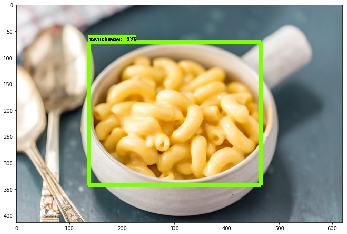
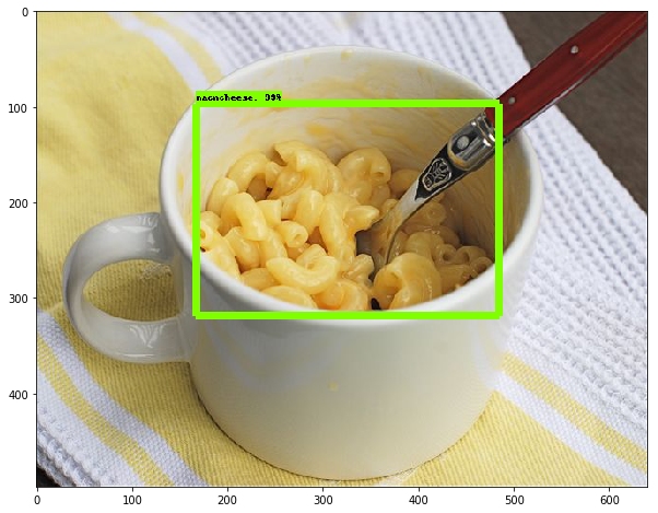
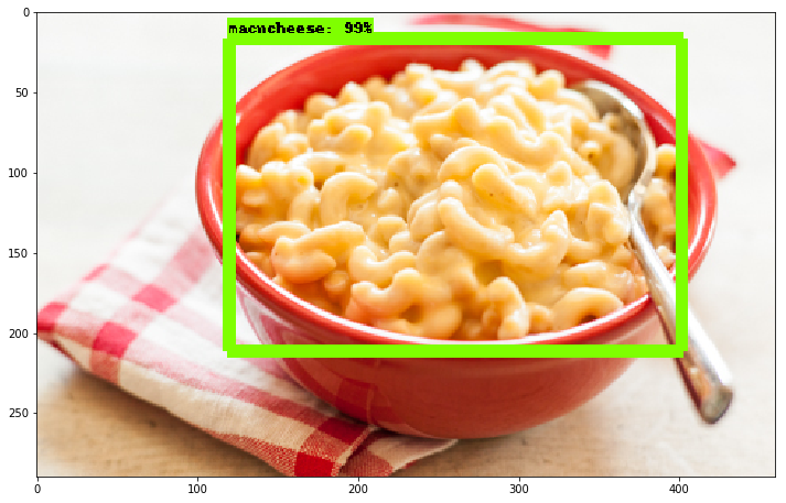
7. Object Detection API(결과)
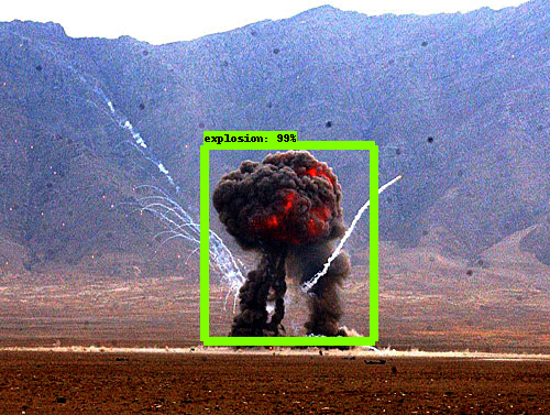
Train Image Count : 67 장
Train Step : 약 5000
loss: 약 0.9
프로젝트 폭발 오브젝트 탐지 시험을 간단하게 완료 하였다.
생각보다 적은량의 이미지로 학습을 적게 하여도 생각보다 꽤 탐지율이 괜찮게 나왔다고 생각한다.
다음 스텝은 Object Detection API 사용되는 모델들은 90 Object에 대한 학습된 모델들이다. COCO 트레이닝
셋에서 사람만 학습하여 모델을 만드는 과정을 진행해야 한다. 이를 진행함과 동시에 부족한 부분을 채워 나가도록하자.